Vertical Lagrangian remapping

Date: 18/06/2026.

Presenter: Angus Gibson (@angus-g).

With generalised vertical coordinates (GVC), we know that vertical velocities permit a range of grid evolution from fully Lagrangian (zero dia-surface transport) to fully Eulerian (zero grid velocity). In MOM6, the dynamics are written in the fully Lagrangian sense: the GVC \(s\) follows fluid elements so that the dia-surface volume flux \(w^{(\dot{s})} = 0\).

If the model is using a purely Lagrangian coordinate, how do we have any control over it? In general, these coordinates drift to a less useful representation of the water column. For example, volume injection at the surface would inflate the upper-most layer, losing resolution for the representation of boundary layer processes. Even more simply, there is indeed irreversible mixing across surfaces that must be captured somehow.

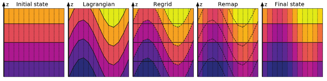
The method has three steps:

1. the Vertical Lagrangian step: evolve the model with a purely Lagrangian generalised coordinate;
2. the Vertical Regrid step: explicitly set the generalised coordinate;
3. the Vertical Remap step: ensure consistency between the ocean state and the new coordinate.

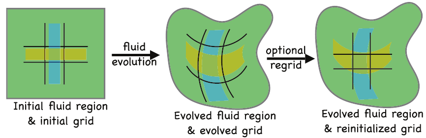
The Vertical Regrid step is where we have the most freedom and flexibility. At this stage, we explicitly set the generalised coordinate \(s(x,y,z,t)\). The choice is arbitrary: it could be predetermined (like a fixed geopotential or terrain-following coordinate); state-dependent (following particular isopycnals by solving for density levels); or even evolutionary (relaxing the current field toward some target value). In fact, you could even change the number of vertical levels!

There is a slight issue after the Vertical Regrid step: the underlying ocean state is no longer consistent with the GVC. The Vertical Remap step fixes this by interpolating (or extrapolating) the state onto the new grid. In the continuous limit, this doesn't change the ocean state. However, since we have limited resolution there is necessarily a spurious change to the state due to interpolation error. Ideally, this numerical mixing is reduced while integrated quantities are conserved.

There are two big advantages to using this method:

1. There is no vertical CFL limit! As long as the remapping can handle interpolation over more than a single cell, the target grid can be arbitrary.
2. Grid evolution can occur on a different timestep to state evolution. You may take several Lagrangian timesteps before performing the regrid/remap steps. Particularly with several tracers (as with BCG), this may give some performance improvements.

A third advantage is that there is a built-in method for remapping the state onto an arbitrary grid, which is useful for diagnostics. You may have a lower-resolution diagnostic grid, or want density-space diagnostics, etc.