Generalised vertical coordinates

Date: 11/06/2026.

Presenter: Andy Hogg (@AndyHoggANU).

In a z-level model, we have vertical velocities, \(w\), which passes through coordinate interfaces.

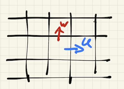
In this case, we can write \(w\) from

\[ \frac{\partial w}{\partial z} = - \nabla \cdot \mathbf{u} \]

Conversely, in the stratified shallow water equations the vertical velocity is entirely associated with the vertical motion of the interface itself. We can call this \(w_{\mathrm{grid}}\).

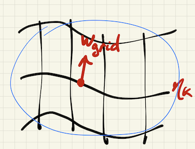
Note that \(w_{\mathrm{grid}}\) has a contribution from both the local rate of change of the interface and an advective component:

\[ w = w_{\mathrm{grid}} = \frac{\partial \eta_k}{\partial t} + \mathbf{u} \cdot \nabla \eta_k \]

In a nutshell, generalised vertical coordinates aims to enable both a cross-interface velocity and the movement of the interface itself. We would take a scalar field \(s(x,y,z,t)\), where \(s\) is monotonic in \(z\) (actually, its derivative cannot be zero). Then, to first order, we can calculate the diasurface flux across a surface of constant \(s\) to be

\[ w^{(\dot{s})} \approx w - w_{\mathrm{grid}} \]

That is, the diasurface velocity, \(w^{(\dot{s})}\), and the velocity of the interface, \(w_{\mathrm{grid}}\), combine to make up the actual vertical velocity.

However, this is a caveat here, and that is the ``\(\approx\)'' in the equation above. In fact, the situation is made more complex by geometric effects (basically, the coordinate interface not being flat). For a full treatment of this derivation, I refer you to Appendix D of the Griffies et al. (2020) paper on ALE. There, they show that we can write

\[ w^{(\dot{s})} \, dA = \mathbf{\hat{n}} \cdot (\mathbf{v} - \mathbf{v_{\mathrm{grid}}}) \, dS, \]

where \(dS\) is the area of the surface over the grid cell, \(dA\) is the projection of that area onto a flat plane, \(\mathbf{\hat{n}}\) is the unit normal and \(\mathbf{v}\) is the 3D velocity field.

I won't reproduce the full derivation here, but to summarise, a little trigonometry allows the above equation to be written as

\[ w^{(\dot{s})} = \frac{dz}{ds} \frac{Ds}{Dt} \]

\[ w^{(\dot{s})} = \frac{dz}{ds} (\frac{\partial s}{\partial t} + \mathbf{v} \cdot \nabla s) \]

...

\[ w^{(\dot{s})} = w - (\frac{\partial z}{\partial t} + \mathbf{u} \cdot \nabla_s z) \]

You may note that this final equation is similar in form to the approximate equation above, except that there is an additional advection term at the end.

In summary, generalised vertical coordinates are mathematically complicated, but the principle is relatively simple: both vertical Lagrangian motion of the grid and dia-surface flux through the coordinate interface is permitted. Importantly, GVCs are a nice framework to help understand the logic of vertical Lagrangian remapping, which Angus will talk about next week ...